
Checks on Photometry
Systematic errors
Whenever possible, the photometry of the MegaPipe images is directly tied to the SDSS photometry. There are a thousand or so standards in every field. Thus, the systematic errors for these images are effectively nil with respect to the SDSS. The systematic errors in the SDSS are quoted as 2-3% (Ivezic, et al., 2004).
The systematic errors for MegaPipe images not in the SDSS are limited by the quality of the Elixir photometric calibration. By comparing the Elixir photometric calibration to the SDSS over a large number of nights, the systematic errors are can estimated. The night-to-night scatter for is typically 0.02 to 0.03 magnitudes. Adding in quadrature SDSS systematic error (0.025 mags) to the systematic error in transferring from the primary to secondary standards (0.025 mags) we get 0.035 magnitudes of total systematic error.
External comparisons
Some MegaPipe groups lie within the SDSS. This makes it possible to directly compare the magnitudes in those fields to an external reference. The figure below shows the difference between the SDSS (transformed to the MegaCam system as described on the MegaCam ugriz filter page) and a MegaPipe image for the 5 bands. The agreement is very good. There is no evidence for systematic shifts greater than 0.01 magnitudes. There is also relatively little scatter (at least at moderate magnitudes). This argues that the colour terms in the SDSS-MegaCam transformation are fairly accurate.
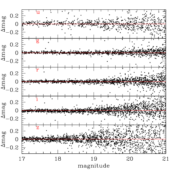
The comparison above applies to images that were photometrically calibrated using the SDSS, so it is not surprising that there are no residuals. As a test of the Elixir calibration, a number of groups lying within the SDSS were stacked using only the Elixir zero-points. The photometric residuals between the resulting stacks and the SDSS were typically 0.03 magnitudes, consistent with the photometric residuals between the individual (non-stacked) images and the SDSS.
Internal consistency
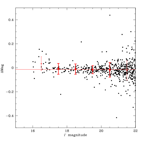
The internal consistency is checked by comparing catalogues from different groups. Groups occasionally overlap each other; even if they only overlap by a arcminute or two, there are usually several hundred sources in common in the two catalogues. Since groups are reduced independently of each other, and since often the data were taken on different nights, comparing the magnitudes of objects common to two groups makes it possibly to check the internal consistency.
Any systematic errors will show up as an offset in the median of the difference in magnitudes between the two groups, as shown in the figure below. The offset in this case is -0.014 magnitudes. This same test is applied to all possible pairs of groups where there were more than 100 objects in common between the catalogues. The typical offset was found to be 0.015 magnitudes. This is smaller than the night-to-night variation of the Elixir zero-points (which is 0.03 mags) for two reasons: many groups lie within the SDSS so that their photometric calibration does not depend on the Elixir zero-points; and further, some neighbouring groups were observed on the same night so any systematic error in the Elixir zero-points will be common to both groups.
Star colours
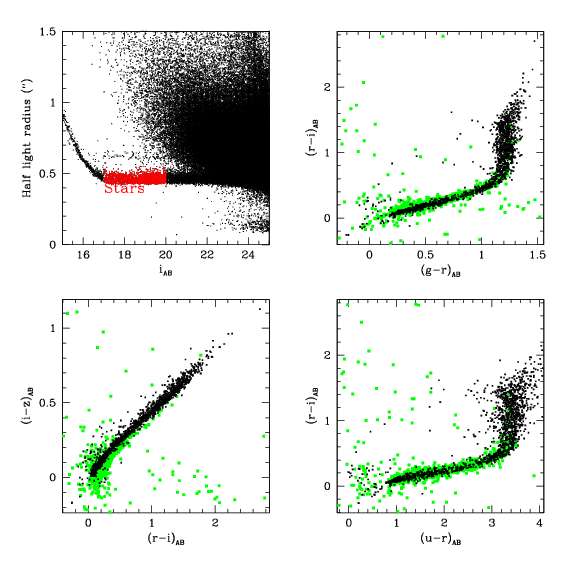
A useful diagnostic of photometry is to examine the colours of stars. Stars have a relatively constrained locus in colour space. Any offsets between the observed and synthetic colours indicates a zeropoint error. This test can be applied to the fields that do not lie in the SDSS and cannot be checked directly.
The top left panel of the figure below illustrates the selection of stars for a typical image. The plot shows half-light radius plotted as a function of magnitude. On this plot, the galaxies occupy a range of magnitudes and radii while the stars show up as a well-defined horizontal locus, turning up at the bright end where the stars saturate. The red points indicate the very conservative cuts in magnitude and radius used to select stars for further analysis.
The other 3 plots show the colours of the stars selected in this manner in black overlaid on top of the transformed SDSS star colours shown in green. No systematic shifts are visible
Limiting magnitudes
The limiting magnitudes of the images are measured in three ways:
- Number count histogram
- 5-sigma point source detection
- Adding fake objects
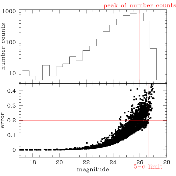
The first method is quite simple, indeed crude. The magnitudes of the objects are sorted into a histogram. The peak value of the histogram, where the number counts start to turn over, is a rough measure of the limiting magnitude of the image.
The second method is also simple. The estimated magnitude error of each source is plotted against its magnitude. In this case, the SExtractor MAG_AUTO or Kron-style magnitude is plotted. At the faint magnitudes typical of MegaCam images, the sky noise dominates the magnitude error. This means that extended objects (which have more sky in their larger Kron apertures) will be noisier for a given magnitude than compact sources. Turning this around, this means that, for a given fixed magnitude error, a point source will be fainter than an extended source. A 5-sigma detection corresponds to a S/N of 5 or, equivalently, a magnitude error of 0.198 magnitudes. Thus, to find the 5-sigma point source detection limit, one finds the faintest source whose magnitude error is 0.198 magnitudes or less. It must be a point source, therefore, its magnitude is the 5-sigma point source detection limit. A more refined approach would be to isolate the point sources, by using the half-light radius for example. In practice, the quick and dirty method gives answers that are correct to within 0.3 magnitudes or so, which is accurate enough for many purposes. This is the value that is given in the image headers for the MAGLIM keyword.
The figure below illustrates these methods. The top panel shows the number count histogram. The number counts peak at 26 in magnitude as shown by the vertical red line.
The bottom panel shows magnitude error plotted against magnitude. The horizontal red line lies at 0.198 magnitudes. The vertical red line intersects the horizontal line at the locus of the faintest object with a magnitude error less than 0.198 magnitudes. The magnitude limit by this method is 26.6 magnitudes.
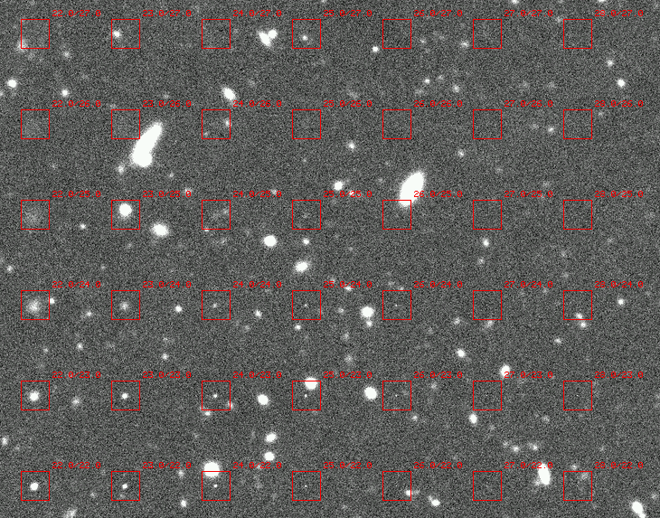
The final way the limiting magnitudes of the images are tested is by adding fake galaxies to the images and then trying to recover them using the same parameters used to generate the real image catalogues. The fake galaxies used were taken from the images themselves, rather than adding completely artificial galaxies. A set of 40 bright, isolated galaxies are selected out of the field and assembled into a master list. Postage stamps of these galaxies are cut out of the field. The galaxies are faded in both surface brightness and magnitude through a combination of scaling the pixel values and resampling the images.
To test the recovery rate at a given magnitude and surface brightness, galaxy postage stamps are selected from the master list, faded as described above to the magnitude and surface brightness in question, and then added to the image at random locations. SExtractor is then run on new image. The fraction of fake galaxies found gives the recovery rate at that magnitude and surface brightness, An illustration of adding the galaxies is shown below. The same galaxy has been added multiple times to the image. The galaxy has been faded to various magnitudes and surface brightnesses. The red boxes contain the galaxy. The boxes are labeled by mag/surface brightness. Note the galaxy at i=23, μi=25 accidentally ended up near a bright galaxy and is only partially visible. Normally of course, the galaxies are not placed in such a regular grid.
To test the false-positive rate, the original image is multiplied by -1; the noise peaks became noise troughs and vice-versa. SExtractor is run, using the same detection criteria. Since there are no real negative galaxies, all the objects thus detected are spurious.
The magnitude/surface brightness plot below shows the results of such simulations. The black points are real objects. The bottom edge of the black points is the locus of point-like objects. The green points show the false-positive detections. The red numbers show the percentage of artificial galaxies that were recovered at that magnitude/surface brightness. The blue contour lines show the 70% and 50% completeness levels.
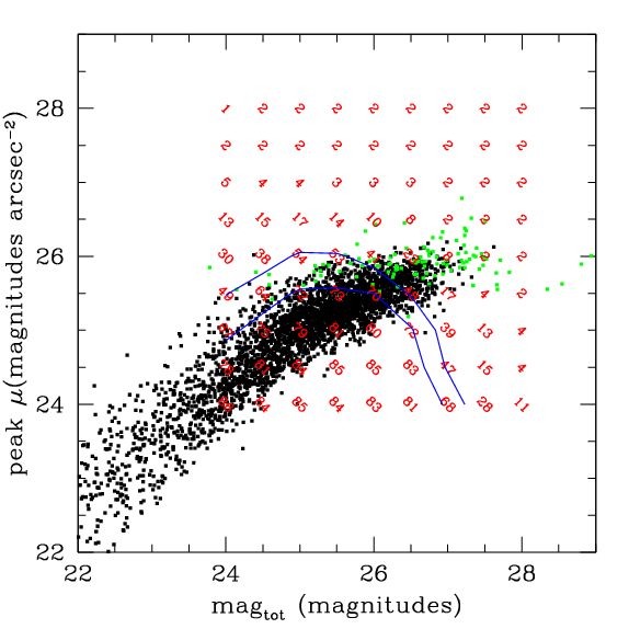
Deriving a single limiting magnitude from such a plot is somewhat difficult. The cleaner cut in the false positives seems to be in surface brightness. Extended objects become harder to detect at brighter magnitudes whereas stellar objects are detectable a magnitude or so fainter.
Note that this plot is of limited usefulness in crowded fields. In this case, an object may be missed even if it is relatively bright because it lies on top of another object. However, the objects in crowded fields are almost always stellar. This suggests the use of the DAOphot package rather than using the SExtractor catalogs provided as part of MegaPipe.
- Date modified: